
Demand Forecasting with Python and Snowflake
10.04.2024Demand forecasting

Demand forecasting is a critical business process which specifically focuses on predicting the quantity of goods or services that customers are likely to purchase within a specific time frame. In order to make an accurate forecast, it is crucial to choose the appropriate forecasting model, which largely depends on the nature of the data. Therefore, before initiating the forecasting process, it is important to analyse and understand the dataset.
As sample data, I have used Time Series dataset containing monthly sales data for the period from July 1991 to June 2008. Dataset can be found here Time Series Analysis Dataset (kaggle.com). I furtherly uploaded this dataset to my Snowflake demo account, to demonstrate real life scenario where we want to access live data from the database. Later, the results of the forecast are uploaded into a Snowflake table, allowing other users to access and use that data.
Connecting to Snowflake and preparing the environment
I am using Python 3.11.5 version, and Visual Studio Code for my IDE. To connect to Snowflake, we need the Snowflake Connector for Python, which serves as an interface for developing Python applications that can connect to Snowflake. You can read more here: Snowflake Connector for Python | Snowflake Documentation. To install this let’s run pip install:
pip install snowflake-connector-python

#If you don't have pandas library already installed, you should run:
pip install "snowflake-connector-python[pandas]"
After installing the connector, we need to connect to the Snowflake account. First, we need to import the snowflake.connector module, and then we need to get login information from environment variables, the command line, a configuration file, or another appropriate source.
import snowflake.connector

#Connect is the API object used to connect to Snowflake
conn = snowflake.connector.connect(
 user=USER,
 password=PASSWORD,
 account=ACCOUNT,
    session_parameters={
        'QUERY_TAG': 'Forecasting',
    }
)
print("success in connecting", conn)
Let’s now prepare the environment. For this purpose, I have created a new role, a new database and a new schema and granted necessary privileges.
#Cursor is the API object used for executing DDL/DML statements and queries
cur = conn.cursor()

#create a custom role
cur.execute("use role useradmin;")
cur.execute("create role data_scientist;")

#grant the role to myself
cur.execute("set my_user = current_user();")
cur.execute("grant role data_scientist to user identifier($my_user);")

#create a database, schema, and grant privileges
cur.execute("use role sysadmin;")
cur.execute("create database forecasting_db;")
cur.execute("grant usage on database forecasting_db to role data_scientist;")
cur.execute("create schema sales_schema;")
cur.execute("grant all on schema sales_schema to role data_scientist;")
cur.execute("grant usage on warehouse compute_wh to role data_scientist;")
#Use created role, database, schema, and WH
cur.execute("use role data_scientist;")
cur.execute("use warehouse compute_wh;")
cur.execute("use database forecasting_db;")
cur.execute("use schema sales_schema;")
Let’s import all necessary libraries:
import pandas as pd
# plotting data - matplotlib
from matplotlib import pyplot as plt
# Seasonality decomposition
from statsmodels.tsa.seasonal import seasonal_decompose

# holt winters - triple exponential smoothing
from statsmodels.tsa.holtwinters import ExponentialSmoothing

from sklearn.metrics import mean_absolute_error, mean_squared_error

import matplotlib.dates as mdates
from datetime import datetime
To read the data from Snowflake into pandas DataFrame, we should use a Cursor to get the data and then call fetch_pandas_all() cursor method.
cur.execute("select * from sales_data;")

sales_data = cur.fetch_pandas_all()
#Let's inspect the data
print(sales_data.shape)
print(sales_data.head())
print(sales_data.dtypes)

#Let's convert date_month column into datetime type
sales_data["DATE_MONTH"] = pd.to_datetime(sales_data["DATE_MONTH"])

#Let's also visual the data
plt.plot(sales_data["DATE_MONTH"], sales_data["SALES"]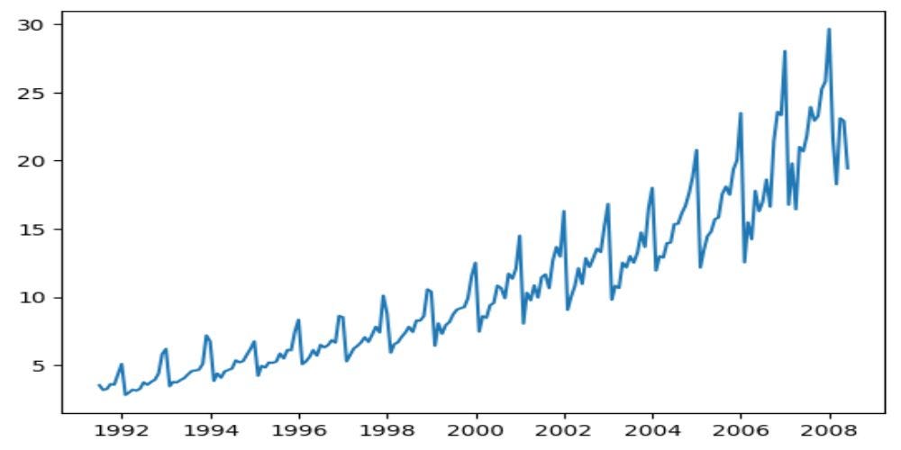
Decomposing the time series
Even though we can clearly see trend and seasonal components in the data by looking at the Figure 1, let’s also decompose the time series to get better understanding about seasonal, level, and trend components:
#I will use multiplicative model, which is appropriate when the seasonality effect increases or decreases proportionally with the overall trend
decompose = seasonal_decompose(sales_data["SALES"], period=12, model = "multiplicative")
decompose.plot()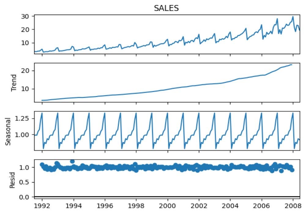
Figure 2 shows us each component individually. In the second plot we can clearly see an exponentially growing trend. The third plot shows a regular seasonal pattern that repeats itself over time. The bottom plot shows the residuals, i.e. the component of the data that is not explained by the trend and the seasonal components. The residuals here look quite stable and do not show any obvious patterns, suggesting that the model has captured the information in the data quite well.
Let’s now quickly check for outliers in the data:
import numpy as np

def outlier_function(sales):
    first_qunatile = np.quantile(sales, 0.25)
    third_qunatile = np.quantile(sales, 0.75)
    IQR = third_qunatile - first_qunatile
    lower_outlier = first_qunatile - IQR * 1.5
    upper_outlier = third_qunatile + IQR * 1.5

    return lower_outlier, upper_outlier
#Let's do outlier test
result = outlier_function(sales_data["SALES"])

print(sales_data[sales_data["SALES"] <= result[0]]) #are there lower outliers
print(sales_data[sales_data["SALES"] >= result[1]]) #are there upper outliers
The results of this function show us that there are no lower outliers, but that there are two upper outliers in January 2017 & January 2018. However, these are the months where seasonal effect has the highest influence, and as we have strong increasing trend, these “outliers” might be justified. Let’s see if the forecasting model will recognize these “outliers”:
#split the data into training and test set
split_index = int(0.8 * len(sales_data))

training_data = sales_data[sales_data.index <= split_index]
test_data = sales_data[sales_data.index > split_index]
We should now choose appropriate forecasting model that aligns with the characteristics of the dataset. Since we have strong trend and seasonal components I will use Triple Exponential Smoothing (Holt-Winters) forecasting model. For this model, we must choose adequate parameters for Alpha, Beta, and Gamma which controls level, trend, and seasonal component respectively. Also, we need to specify whether the trend and seasonal components are multiplicative or additive.
Since we want to be accurate and efficient, I created a function that will loop through different set of parameters and choose the most optimal ones according to Mean Absolute Percentage Error (MAPE).
def Holt_Winters(TrainData, TestData, SalesColumn, SeasonPeriod):

    #values for alpha, beta, and gamma should range from 0 to 1.
    alpha_values = [int(i) / 10 for i in range(1, 11)]
    beta_values = [int(i) / 10 for i in range(1, 11)]
    gamma_values = [int(i) / 10 for i in range(1, 11)]
    seasonality_types = ["additive", "multiplicative"]
    trend_types = ["additive", "multiplicative"]
    best_mape = float('inf')
    best_params = {}

    # Iterate through parameters
    for alpha in alpha_values:
        for beta in beta_values:
            for gamma in gamma_values:
                for seasonality_type in seasonality_types:
                    for trend_type in trend_types:
                        try:
                            # Fit Holt-Winters model
                            model = ExponentialSmoothing(TrainData[SalesColumn], seasonal = seasonality_type,
                                                            seasonal_periods = SeasonPeriod,
                                                            trend = trend_type,
                                                            )
                            hw_model = model.fit(smoothing_level = alpha,
                                                smoothing_trend = beta,
                                                smoothing_seasonal = gamma,
                                                )

                            # Make forecast
                            hw_forecast = hw_model.forecast(len(test_data))

                            # Calculate forecasting error metrics
                            hw_metrics = {
                                'MAE': mean_absolute_error(TestData[SalesColumn], hw_forecast),
                                'MAPE': mean_absolute_error(TestData[SalesColumn], hw_forecast) / TestData[SalesColumn].mean() * 100
                            }

                            # Check if current combination yields a better MAPE
                            current_mape = hw_metrics["MAPE"]
                            if current_mape < best_mape:
                                best_mape = current_mape
                                best_mae = hw_metrics["MAE"]
                                best_params = {'Alpha': alpha, 'Beta': beta, 'Gamma': gamma, 'Seasonality': seasonality_type, 'Trend': trend_type, 'MAPE':best_mape, 'MAE':best_mae}
                        except:
                            pass #if pass, it means that combination of parameters resulted in NaN values
    return best_params

#Period = 12 since we have montly data
Holt_Winters(training_data, test_data, "SALES", 12)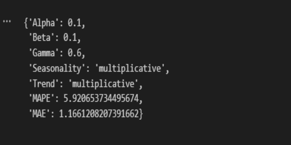
Figure 3 shows the most optimal parameters for our model. Multiplicative trend and seasonality are expected. A multiplicative trend suggests that changes in a time series are proportional to its current value, meaning that as the series grows, the magnitude of its fluctuations tends to grow as well. Multiplicative seasonality indicates that the seasonal swings are also proportionate to the trend, so during periods of higher values, the seasonal peaks and troughs become more pronounced.
Alpha, Beta, and Gamma parameters can have value from 0 to 1. The smaller the value, the less weight is assigned to recent observations, making the forecast more smooth. On the other hand, large value of parameters gives more weight to the recent observations, making the forecast more responsive to the recent changes. MAPE of 5.92 indicates 94.08% accuracy (100-MAPE), which is desirable result.
#let's do the forecast and visual the differences
model = ExponentialSmoothing(training_data["SALES"], seasonal="multiplicative",
                                                            seasonal_periods=12,
                                                            trend = "multiplicative")
hw_model = model.fit(smoothing_level = 0.1,
                    smoothing_trend = 0.1,
                    smoothing_seasonal = 0.6)

# Make forecast
hw_forecast = hw_model.forecast(len(test_data))

#To easily compare the numbers
#test_data2 = test_data
#test_data2["forecasted"] = hw_forecast
#test_data2["difference"] = test_data["sales"] - hw_forecast

#Plot the forecast
fig, ax = plt.subplots()
ax.plot(training_data["DATE_MONTH"], training_data["SALES"])
ax.plot(test_data["DATE_MONTH"], test_data["SALES"])
ax.plot(test_data["DATE_MONTH"], hw_forecast)
plt.legend(['TRAIN', 'TEST', 'Holt-Winters forecast'])
plt.title("Holt-Winters Triple Exponential Smooting")
plt.show()
Figure 4 clearly show how forecasting model managed to capture trend and seasonal patterns. As mentioned, the forecasting model resulted in 94.08% accuracy. Before, the outlier function indicated that values in January 2017 & January 2018 are outliers. However, we see that the model also forecasted these high values. Therefore, we can conclude that these sales values are not outliers but true representation of variability in the data, justified by presence of strong trend and seasonal components. We can now take a closer look to a forecasted part to observe the differences:
plt.plot(test_data["DATE_MONTH"], test_data["SALES"])
plt.plot(test_data["DATE_MONTH"], hw_forecast)
plt.legend(['Actual values', 'Holt-Winters forecast'])
plt.xticks(fontsize=7.5)
plt.show()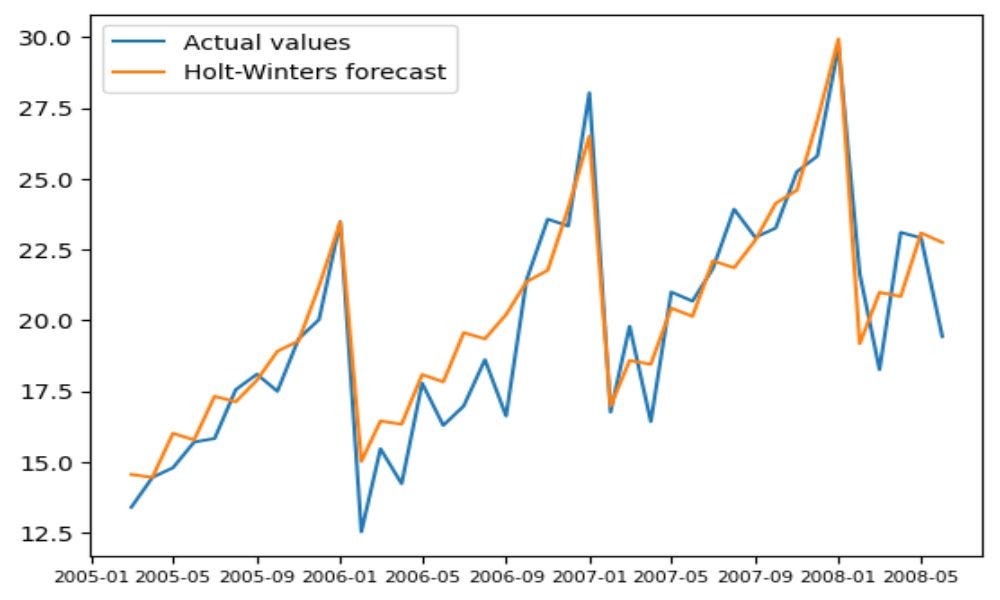
Again, we see how model managed to capture data components correctly.
We can now do the actual forecast for the next period and then save the data into Snowflake.
model = ExponentialSmoothing(sales_data["SALES"], seasonal="multiplicative",
                                                            seasonal_periods=12,
                                                            trend = "multiplicative")
hw_model = model.fit(smoothing_level = 0.1,
                    smoothing_trend = 0.1,
                    smoothing_seasonal = 0.6)

# Make forecast
hw_forecast = hw_model.forecast(steps = 18) #1.5 year forecast
dates = pd.date_range(start='2008-07-01', end='2009-12-01', freq='MS')

Forecast = pd.DataFrame(dates, columns=["DATE_MONTH"])
Forecast["FORECASTED_VALUES"] = hw_forecast.values

plt.plot(sales_data["DATE_MONTH"], sales_data["SALES"])
plt.plot(Forecast["DATE_MONTH"], Forecast["FORECASTED_VALUES"])
plt.legend(['Historical data', 'Forecasted demand'])
plt.xticks(fontsize=7.5)
plt.show()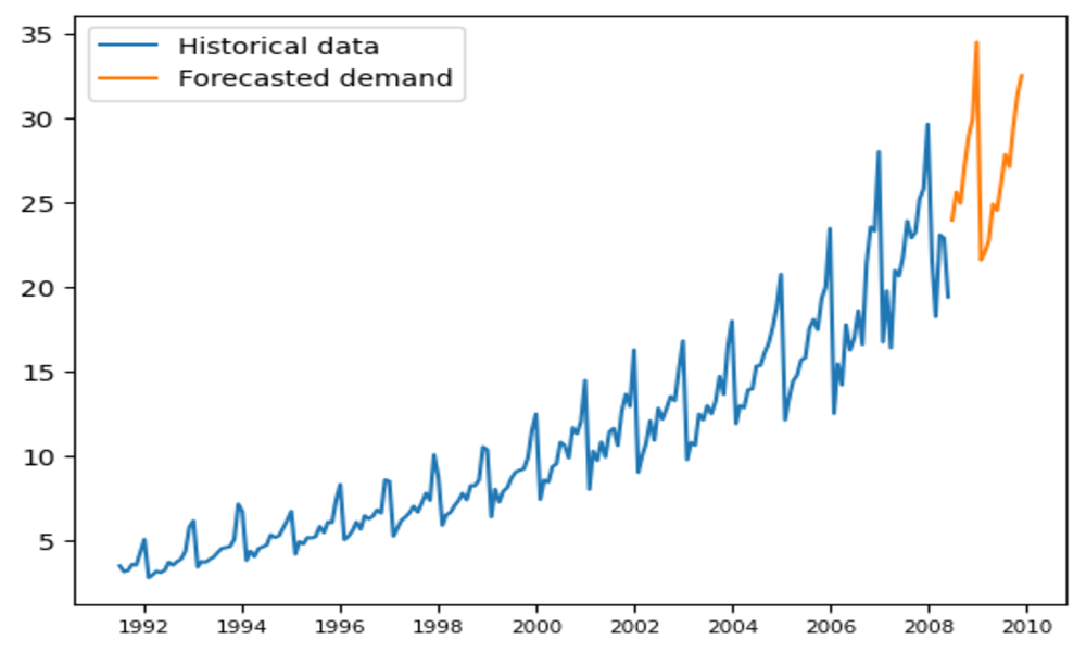
Again, we see that the forecasting model successfully recognized seasonal and trend patterns in the data.
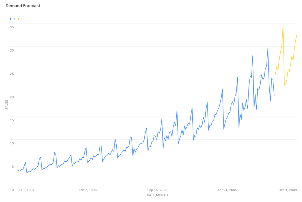
Let’s now load the forecast into Snowflake table, so it is easily accessible to other users.
snowflake.connector.pandas_tools import write_pandas
from snowflake.connector.pandas_tools import pd_writer

#Adjust the data for easier conversion
Forecast["DATE_MONTH"] = Forecast["DATE_MONTH"].astype(str)
Forecast["FORECASTED_VALUES"] = Forecast["FORECASTED_VALUES"].round(2)

cur.execute("CREATE OR REPLACE TABLE FORECASTED_DEMAND( "
            "DATE_MONTH date, FORECASTED_VALUES float "
            ");"
            )
# Write the data from the DataFrame to the Snowflake table called Forecasted_demand.
success, nchunks, nrows, _ = write_pandas(conn, Forecast, 'FORECASTED_DEMAND')
#Close the cursor and connection
cur.close()
conn.close()
Other users can furtherly visualise the forecast data directly on Snowflake using dashboards.
Conclusion
Demand forecasting with Python and Snowflake highlights the significance of selecting a suitable forecasting model and thoroughly analyzing the dataset to ensure accurate predictions. By leveraging the Snowflake Connector for Python and implementing the Triple Exponential Smoothing (Holt-Winters) model, I have demonstrated an efficient and precise forecasting process with a remarkable 94.08% accuracy. This case study not only showcases the potential of combining advanced analytics with cloud data warehousing but also emphasizes the importance of accessibility and collaboration, as forecast results are made readily available for other users within Snowflake. This approach to demand forecasting serves as an example for businesses looking to optimize their supply chain and inventory management strategies in a data-driven world.

Consultant and Data Engineer
